
If you have tried our two-dimensional sentiment model, you might have noticed that its scores are not only accurate but also sensitive to context, and often better than human performance. The model combines ideas from
- psychological research on emotion with
- DIY sentiment models that were built on top of large language models,
and connects everything together using mathematical convex combinations. After some prompt engineering and optimizing input size, it performed well on real-world data, allowing us to predict patient outcomes immediately after COMP360 psilocybin administration with an AUC of 88%.
If you want to run it yourself, you can just run the code block below:
%%capture
%pip install git+https://github.com/compasspathways/Sentiment2D
from sentiment2d import Sentiment2D
sentiment2d = Sentiment2D()
SST003967 = 'While it’s not quite “Shrek” or “Monsters, Inc.”,' + " it’s not too bad."
valence, arousal = sentiment2d(SST003876)
valence, arousal
(0.7168753743171692, -0.7362477034330368)Psilocybin Therapy and Natural Language Processing (NLP)
COMP360 therapy involves a psilocybin administration session plus one or more preparation sessions prior to the psychedelic experience and at least one integration session afterwards.
Each support session lasts about an hour and is a dialogue between patient and therapist. During the preparation session the conversation focuses around how to be best prepared for the upcoming administration session. During the integration session, the discussion focuses on processing and working through the patient’s psychedelic experience. This dialogue opens up unique possibilities to analyze a participant’s experience using NLP techniques after the session is recorded and transcribed. Our two-dimensional sentiment model is an example of how meaningful information can be extracted from such data.
Two-Dimensional Sentiment
In NLP, sentiment is the emotional tone of the subject matter of a piece of text. It is essentially the textual version of emotion. Generally speaking, quantitative descriptions of emotion come in two flavors: categorical and dimensional. Categorical models run along the lines of “Happy? Yes or no.”
Dimensional models on the other hand treat emotions as living in one or more dimensions. These can deal with questions like “Happy? How happy? Is it a calm happy or an excited happy?”.
Typical, out-of-the-box sentiment analyzers are the categorical sort. They provide an answer to a single question “Positive? Yes or no.” For our work, we wanted the nuance that a dimensional model can provide.
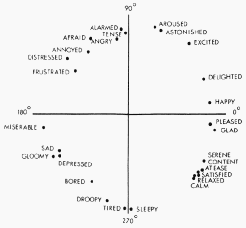
A famous example of a two-dimensional model is Russell’s Circumplex (Russell, 1980). James Russell introduced a two-dimensional model whose x-axis is valence and whose y-axis is arousal. Valence is akin to “positivity”, and arousal is similar to “energy”. For example, “excited” is high in both valence and arousal, whereas “furious“ is low valence and high arousal. Low arousal examples include “depressed” and “grounded”, the first low valence and the second high valence.
Our Two-Dimensional Sentiment
We were able to produce a model that is faithful to Russell’s vision of a two dimensional space of emotions by combining a zero-shot classification model and a trick of mathematics, specifically: convex combinations. The result was a model that scored the emotional content of sentences in a way that agreed with human judgement.
You can find the full code for the model here, but the idea is simple. In the class Sentiment2D, there are two important methods:
- get_utterance_class_scores(self, utterance) which returns the class scores scores of utterance for classes = [“happy”, “angry”, “gloomy”, “calm”] using the BART-MNLI zero-shot classifier.
- get_utterance_valence_arousal(self, utterance) which returns the aggregated scores in two different ways to get numbers called valence and arousal. Specifically, the formulas are:
valence = scores["happy"] + scores["calm"] - scores["angry"] - scores["gloomy"]

arousal = scores["happy"] + scores["angry"] - scores["calm"] - scores["gloomy"]
The intuition behind the valence and arousal scores is that sentiment should capture the positivity/negativity of a specific utterance while the arousal should capture its excitement/calmness. At first pass, this suggests that we might use classes “positive”, “negative”, “excited”, and “calm”, and then use formulas like
valence = scores["positive"] - scores["negative"]

arousal = scores["excited"] - scores["calm"].
This would also produce a range of possible values in the 2×2 plane with coordinates between -1 and 1. However, we quickly found that a slightly less direct method worked better.
Another way to fill out the 2×2 square with coordinates between -1 and 1 is to use convex combinations of the four corners (1, 1), (-1, 1), (-1, -1), and (1, -1). A convex combination is a vector sum
$$ w_{++} (1,1) + w_{-+} (-1,1) + w_{-\,-} (-1,-1) + w_{+-} (1,-1) $$
where the weights are non-negative and sum to 1. Collecting this sum as a single vector gives
$$ (w_{++}+w_{+-}-w_{-+}-w_{-\,-}\ , \quad w_{++}+w_{-+}-w_{+-}-w_{-\,-})$$
Setting
w_{++} = scores["happy"]
w_{-+} = scores["angry"]
w_{--} = scores["gloomy"]
w_{+-} = scores["calm"]
calculates (after rearranging terms) valence and arousal as the first and second coordinates of the vector. Putting everything together, we have
(valence, arousal) =     scores["happy"] (1,1) + scores["angry"] (-1,1)
                    + scores["gloomy"] (-1,-1) + scores["calm"] (1,-1).
Convex combinations can also be interpreted as the center of mass. So for us, the valence and arousal represent the center of mass of four point masses; namely
(1, 1), (-1, 1), (-1, -1), and (1, -1)
whose masses are simultaneously proportional to the
scores[“happy”], scores[“angry”], scores[“gloomy”], and scores[“calm”].
A great way to see the model in action is the plot of every utterance in a real therapy session. For instance, the figure below plots the sentiment scores for a well-known session between the therapist Carl Rogers and his patient Gloria (transcript and video are available).
*Sentiment scores for the utterances from a session between the therapist Carl Rogers and his patient Gloria. Carl’s utterances are in blue and Gloria’s in orange. The size of the dot represents the length of the utterance.
We’ll now get into the specifics how each of the scores that go into the valence and arousal computation are calculated.
Zero-Shot Classification with BART

The heavy lifting in our model is done with the BART-MNLI zero-shot classifier. A zero-shot classifier is a model that takes a list of classes and a piece of text, and returns a list of scores, one for each class. The score of a given class is the probability that the content of the text is about that class. For example, using the facebook/bart-large-mnli model on the classes [“scratch”, “arm’s off”] for the text “It’s just a flesh wound.” yields the following :
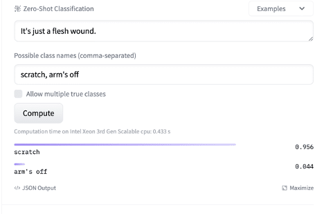
*Image courtesy of Hugging Face and their BART-MNLI interface.
**We note that this settles a debate going back to least the time of King Arthur.
The term “zero-shot” comes from the fact that the model allows one to produce a classifier on any arbitrary classes with zero additional training or tuning. In the larger picture, it lies in the realm of “transfer learning” where a model trained on one task is used to solve a different task. Zero-shot learning lies at the extreme end of what is called “few-shot” learning, where a model is adapted to a new task after retraining/tuning on a “few” examples. This May 2020 blog post by Joe Davidson has additional discussion.
The BART-MNLI model pulls off this feat by using a trick devised by Wenpeng Yin, Jamaal Hay, and Dan Roth in 2019. BART-MNLI is the pretrained BART model tuned using the multi-genre natural language inference (MNLI) dataset. The MNLI dataset is made up of pairs of passages of text, the first called a premise and the second called a hypothesis. These pairs are labeled with one of three labels:
- whether the hypothesis can be inferred from the premise (otherwise known as “entailment”),
- whether the hypothesis and premise are contradictory (“contradiction”),
- neither.
Once tuned, the BART-MNLI model becomes a zero-shot classifier by using an appropriate “hypothesis”. For example, to tell if some text is about politics, one takes that specific text block as the premise (for example: Who are you voting for in 2024) and This text is about politics as the hypothesis. The model would then output a probability score if there is an “entailment”. A simplified version of this process is described well (and with code!) in this post.
BART Architecture and MNLI Tuning
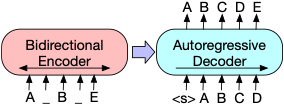
BART itself is structured as a two component model: A bi-directional auto-encoder (in the style of BERT) and an autoregressive decoder (in the style of GPT). To use BART for classification tasks, the final hidden state from the decoder is fed into a linear classifier. A more detailed discussion can be found in the original paper along with the hugging face page.
Once we had settled on using a zero-shot classifier based on a Large Language Model (LLM) we were able to utilize BART’s infrastructure on our moderately sized, unlabeled dataset (approximately 1000 hours of dialog). The importance of making the most out of large pretrained models is an inescapable reality of the current data ecosystem and as we dug into the model and data, we found that there were two important considerations when using BART-MNLI:
- Prompt engineering,
- Briefly, “prompt engineering” involves figuring out the best “prompt/premise” to submit to the model in order to get the desired outcome.
- We tried many different prompts, and ultimately settled on four simple words: “happy”, “angry”, “gloomy”, and “calm”.
- Optimizing string input size.
- Experimentation with text input size is critical. Our first instinct was that a chunk of text containing several sentences would be best. The idea behind that instinct being that the additional context would result in better sentiment scores. Ultimately, we found that the size that worked best was a single sentence.
- We suspect single sentences worked best for two reasons:
- First, the MNLI dataset is made up of pairs of successive sentences, so the single-sentence approach better matched the tuning inputs of BART-MNLI.
- Second, upon examination it was evident that a passage of several sentences could move around between different emotions without having a clearly defined overriding sentiment, thus forcing the model to make an impossible judgement call. Single sentences avoided this problem and resulted in a less ambiguous sentiment score.
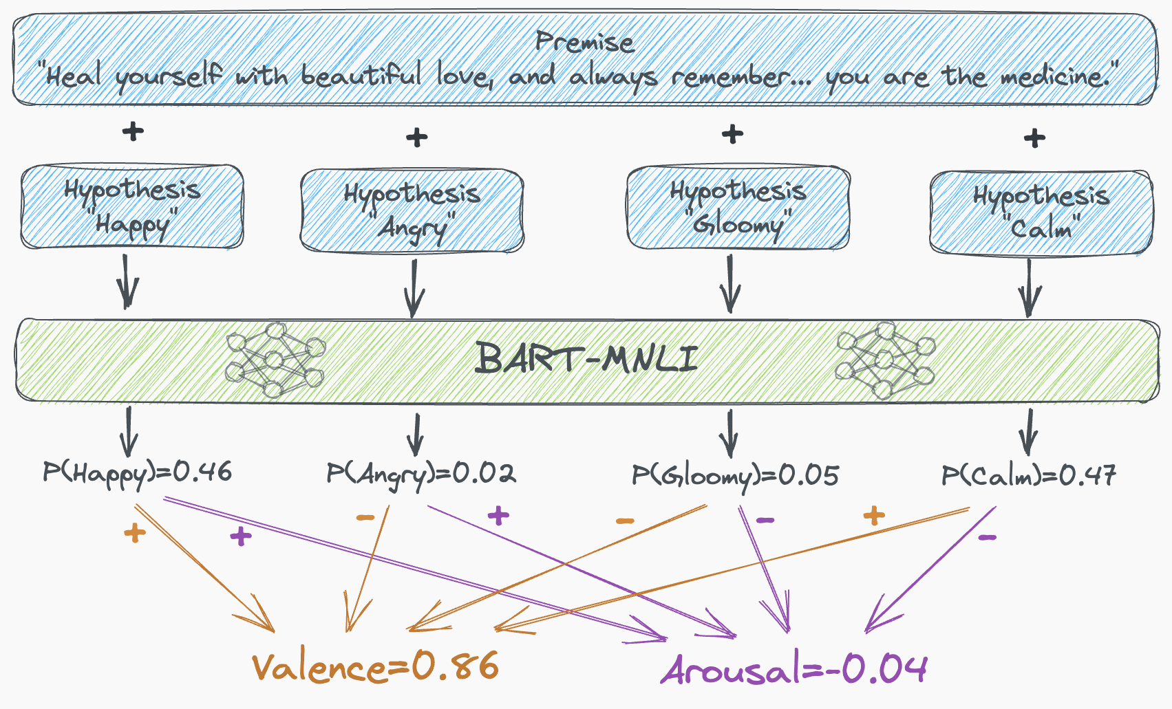
Once we had optimized the two items above, our model was able to score both the valence and arousal for every “utterance” in our transcript. As mentioned, these scores were then used directly as features in our NLP paper mentioned above. A schematic diagram summarizing the full two-dimensional sentiment model pipeline is shown below.
Conclusion
Large language transformer models are making incredible things possible. A clever use of BART has allowed us to take a theoretical psychological model of emotions out of the ivory tower and into the real world. Specifically, our 2D Sentiment model allows a machine learning model to utilize NLP on the dialogue between patient and therapist during the integration session to potentially predict long term patient outcomes and bring precision medicine to mental health care.
Acknowledgements
I’d like to thank Bob Dougherty, Greg Ryslik, Carly Leininger, Starr Jiang and the whole DELTA Research Team for their help on the project and in writing this article.